Visualizations: {Stringr}

Usingdplyr and the stringr::words package, we can demonstrate how to extract information from a dataset. Before we get into anything, let us take a look at a few of the characteristics of the stringr::words dataset.

library(stringr)
library(dplyr)


Attaching package: 'dplyr'

The following objects are masked from 'package:stats':

    filter, lag

The following objects are masked from 'package:base':

    intersect, setdiff, setequal, union

library(ggplot2)
library(forcats)
library(tidytext)
head(stringr::words)

[1] "a"        "able"     "about"    "absolute" "accept"   "account"

words |> 
  summary()

   Length     Class      Mode 
      980 character character

A dataset with 980 words seems like a great tool to have!

You could use it to create arbitrary categories.
You could also use it to get some words that fit a certain criteria.

Example 1: Only Five Letter Words

Using str_match_all we can enter a regular expression that will see match words that only have five characters.

five_letter <- 
  str_match_all(words,pattern = "\\w{5}")

head(five_letter)

[[1]]
     [,1]

[[2]]
     [,1]

[[3]]
     [,1]   
[1,] "about"

[[4]]
     [,1]   
[1,] "absol"

[[5]]
     [,1]   
[1,] "accep"

[[6]]
     [,1]   
[1,] "accou"

Here we encounter two errors:

We want to return a character vector, but right now we have a list.
We are returning words that have 5 letters, but are not exactly only five letters long.

We will need to use unlist() and \\b in order to fix this.

five_letter_fixed <- 
  str_match_all(words, pattern = "\\b\\w{5}\\b") |> 
    unlist()

head(five_letter_fixed)

[1] "about" "admit" "after" "again" "agent" "agree"

The regular expression here does the following:

\\b represents a boundary character. This tells R to look for something to be followed by a space and finished before a space.
\\w tells R to look for a word-character.
{5} tells R to look for a word-character that has a length of exactly 5.
\\b lookd for the second boundary.

Example 2: Finding Words That Start with AEIOU

Here we will use a regular expression that looks for where words start with specific letters.

vowel_words <- 
 str_match_all(words,"^[aeiou].*$") |> 
  unlist()

sample(vowel_words,10)

 [1] "use"     "imagine" "arrange" "every"   "example" "already" "amount" 
 [8] "okay"    "order"   "into"

Great!

The regular expression does the following:

\\b - Looks for boundary
^ - Designates the start of a string.
[aeiou] - Matches the start of the string that is either a,e,i,o,or u.
. - Looks for any character that follows the first match.
* - Looks for an unlimited number of matches until it is told to stop.
$ - Tells R to look for the end of a string.

Most Common Start Letter Used in `stringr::words`

We will need to make stringr::words into a dataframe using tibble().

We need the data in a dataframe so that we can use the different functions in dplyr package.

We use the %>% operator that takes the value on the left and passes it throuh to the right.

word_tbl <- 
  tibble(line=1:length(words),
         words=words)

word_tbl |> 
  summary()

      line          words          
 Min.   :  1.0   Length:980        
 1st Qu.:245.8   Class :character  
 Median :490.5   Mode  :character  
 Mean   :490.5                     
 3rd Qu.:735.2                     
 Max.   :980.0

word_tbl %>% 
  # Create a column of the letter the word starts with
  mutate(sw= str_match_all(words,"^.") |> unlist()) %>% 
  # Group by that new column. Any change we make will be in accordance with this column. 
  group_by(sw) %>% 
# We will use the tally function to count how many observations fall into each category. 
  tally()

# A tibble: 25 × 2
   sw        n
   <chr> <int>
 1 C         2
 2 a        65
 3 b        58
 4 c        83
 5 d        43
 6 e        45
 7 f        54
 8 g        23
 9 h        38
10 i        25
# ℹ 15 more rows

Taking a look at the table we can see that there are two words that start with a capital C. This doesn’t halt the process, but it is worth it to see who the culprits are.

word_tbl %>% 
  mutate(sw=str_match_all(words,"^.") |> unlist()) %>% 
  filter(sw=="C")

# A tibble: 2 × 3
   line words     sw   
  <int> <chr>     <chr>
1   150 Christ    C    
2   151 Christmas C

For our purposes, it is more than okay to change these entries to be lowercase. Conveniently, the stringr package really does have it all!

words <- 
  str_to_lower(words)

word_tbl <- 
  tibble(line=1:length(words),
         words=words)

word_tbl <- 
  word_tbl %>% 
  # Create a column of the letter the word starts with
  mutate(sw= str_match_all(words,"^.") |> 
           unlist()) %>% 
  # Group by that new column. Any change we make will be in accordance with this column. 
  group_by(sw) %>% 
# We will use the tally function to count how many observations fall into each category. 
  tally()

We could look at the table and make some observations, but it would be better to just graph everything!

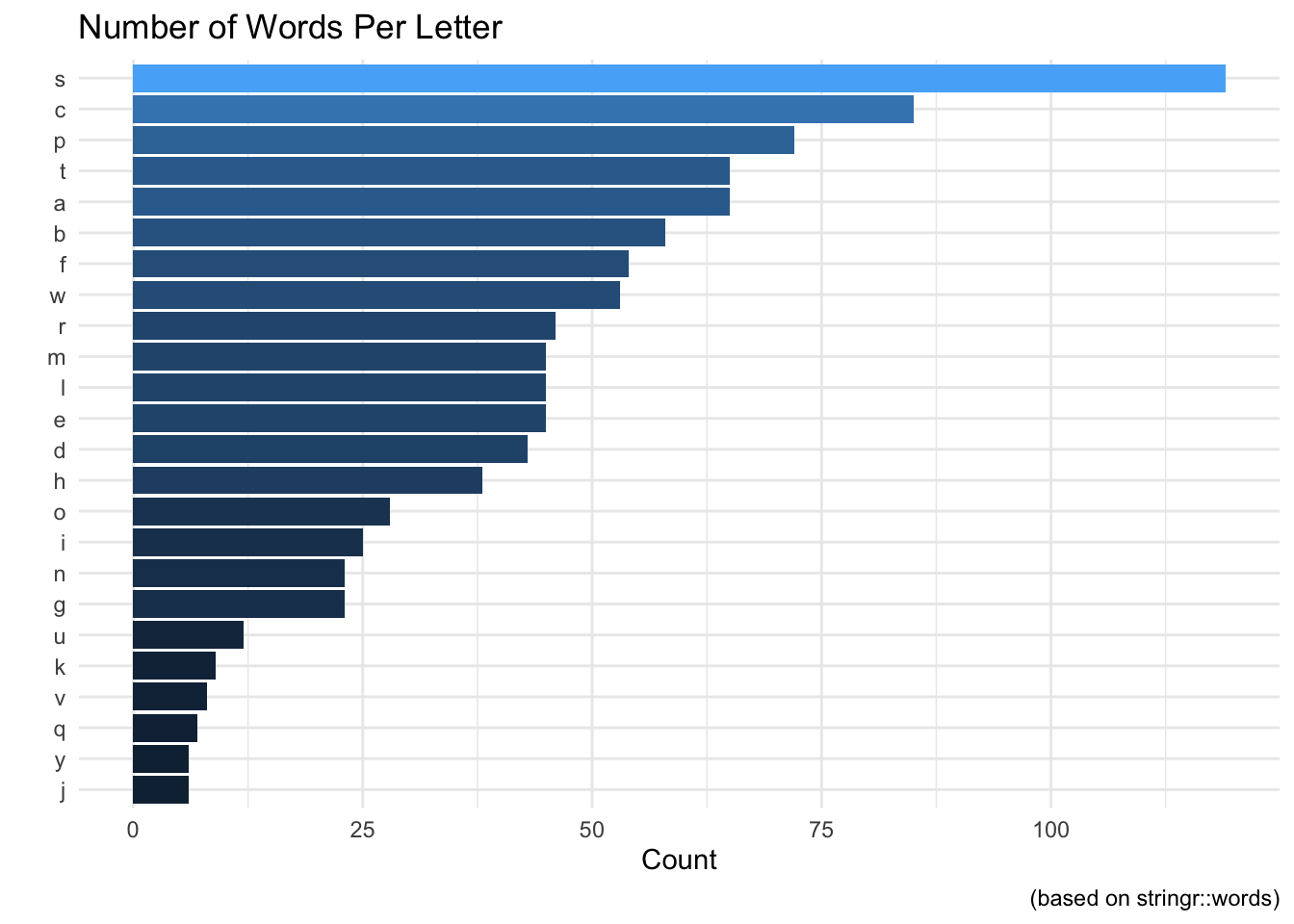
Keep in mind that this list of words is only 980 observations long so there are plenty of missing words. With that being said, what letter is represented the most in the stringr::words vector?

word_tbl %>% 
  ggplot(aes(fct_reorder(sw,n),n,fill=n)) + 
    geom_bar(stat="identity") +
    coord_flip() +
  labs(x="",y="Count",
         title="Number of Words Per Letter",
       caption="(based on stringr::words)") +
    theme_minimal() +
    theme(axis.ticks = element_blank(),
          legend.position = "none")

For example, here is a quick way to create a vector of words and getting their length:

library(stringr)

# Take a sample of 10 observations from the words package
sample_words <- 
  sample(words,10)
# Find the length of each word
sample_words |> 
  str_length()

 [1] 3 5 8 4 7 5 5 3 6 4

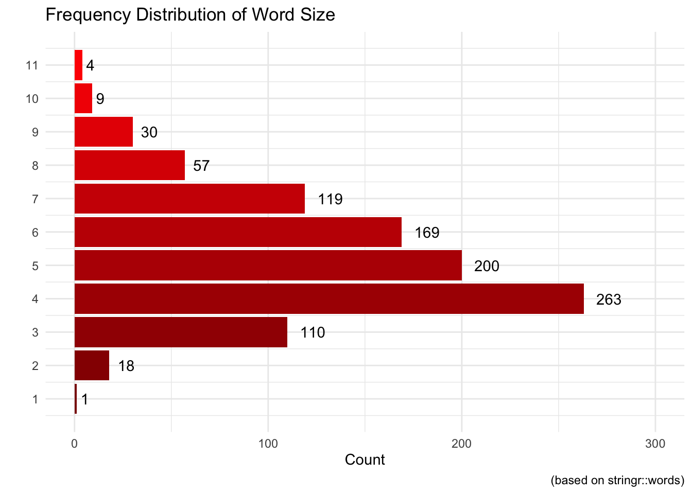
Using this same approach we could find out the number of each letter-sized word in the package.

# X-Axis Values for later
xax <- 1:11
# Create a dataframe to use 
words_t <- 
  tibble(line=1:length(words),
         words=words)
# Create a column with the lengths of the words
words_t <- 
  words_t %>% 
  mutate(string_length=str_length(words)) %>% 
  group_by(string_length) %>% 
  tally()

# Plot the frequencies, flip the coordinates
# use our custom axis labels, remove axis ticks, 
# plot the frequencies on the plot
# label the axes 
words_t %>%
  ggplot(aes(string_length, n, fill = string_length)) +
  geom_col() +
  coord_flip() +
  labs(x = "Length of Word") +
  scale_x_continuous(breaks = xax) +
  theme_minimal() +
  theme(legend.position = "none",
        axis.ticks = element_blank()) +
  scale_fill_gradient(low = "darkred", high = "red1") +
  geom_text(aes(label = n, hjust = -.5)) +
ylim(0, 300) +
  labs(
    x = "",
    y = "Count",
    title = "Frequency Distribution of Word Size",
    caption = "(based on stringr::words)"
  )

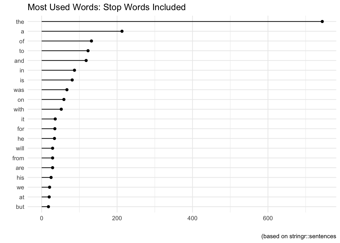
stringr::sentences

sentences_t <- 
  tibble(
    line=1:length(sentences),
    sentence=sentences)

sentences_t_ns <- 
  sentences_t %>% 
  unnest_tokens(word,sentence) %>% 
  group_by(word) %>% 
  count(sort=T) %>% 
  ungroup() %>% 
  slice(1:20) 

sentences_t_ns %>% 
  ggplot(aes(fct_reorder(word,n),n)) + 
    geom_point() + 
    geom_segment(aes(word,xend=word,n,yend=0)) +
    coord_flip() +
    theme_minimal() +
    theme(axis.ticks = element_blank(),) +
    labs(x="",y="",
         title="Most Used Words: Stop Words Included",
         caption="(based on stringr::sentences")

sentences_t_s <- 
  sentences_t %>% 
  unnest_tokens(word,sentence) %>% 
  anti_join(stop_words) %>% 
  group_by(word) %>% 
  count(sort=T) %>% 
  ungroup() %>% 
  slice(1:20)

Joining with `by = join_by(word)`

sentences_t_s <- 
  sentences_t_s %>% 
  ggplot(aes(fct_reorder(word,n),n)) + 
  geom_point() + 
  geom_segment(aes(word,xend=word,n,yend=0)) +
  coord_flip() +
  theme_minimal() +
  theme(axis.ticks = element_blank(),) +
  labs(x="",y="",
       title="Most Used Non Stop_Words",
       caption="(based on stringr::sentences)")
sentences_t_s

Example 1: Only Five Letter Words

Example 2: Finding Words That Start with AEIOU

Most Common Start Letter Used in stringr::words

stringr::sentences

Most Common Start Letter Used in `stringr::words`